


The Chaffin model
Musculoskeletal injuries resulting from physical strain typically share a common cause: the overburdening of bodily structures (such as joints, tendons, tendon sheaths, ligaments, and muscles) due to repetitive and/or excessive strain in improper postures. While numerous ergonomic evaluation methods aim to assess the risk level associated with exertion, it is through the implementation of biomechanical techniques that a more comprehensive and precise evaluation of the risk can be achieved.
Remember...
The most common cause of musculoskeletal injuries is the overloading of structures of the locomotor system due to repeated and/or excessive levels of strain in inappropriate postures.
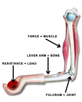
Assessing whether a strain in a specific posture can cause overload in any structure of the locomotor system is a complex task. Biomechanics tackles this challenge by drawing an analogy between the human body and a machine composed of levers and pulleys. In this context, a joint can be viewed as the fulcrum of a lever (a long bone) actuated by a muscle (the force) to counter a resistance (the weight of the limb and any additional load) (Figure 1). By employing this analogy, it becomes possible to apply the laws of physics to determine if joint overloads occur during the execution of an effort.
The stress subjected to the joint arises from two factors: the weight of the body parts and the load, and the moment these forces create at the joint, which must be overcome to maintain the posture. Considering that the moment of a force relative to a point is the vector product of the force vector and the vector distance from the point to the point of force application, and by applying the equations of equilibrium, it is possible to determine the moment and the reaction force on the joint.
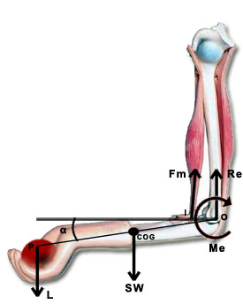
Figure 2 illustrates the elbow joint as an example. The loads borne by the elbow include the weight of the load supported by the hand (L) and the self-weight of the forearm and hand (SW) applied at the limb's center of gravity. Assuming a static position, a reaction force counteracting these loads (Re) and a moment (Me) of equal magnitude but opposite sign to that caused by SW and L must appear at the elbow. By applying the laws of equilibrium, the values of Me and Re can be determined:
Figure 1:
Member-lever analogy
Re = L + SW
Me = L x OP x cos(α) + SW x O COG x cos(α)
Once Me and Re are determined, the next step is to find out whether the values they assume might be harmful to the joint in question. This procedure can be repeated for each joint, thereby identifying if the effort exerted may be detrimental to any of them. To accomplish this, it is necessary to know the maximum recommended value of Mc for each joint.
In the example illustrated in Figure 2, the moment Me counteracts the moment generated in the elbow by the load (L) and the weight of the hand and forearm (SW). The Me moment at the elbow is produced by the flexor muscles located in the arm segment: biceps, brachialis, and brachioradialis. The contraction of this group of muscles generates a force (Fm) through the tendon that connects them to the radius bone, and this force creates the Me moment. Consequently, it can be stated that:
Me = Fm x IO x cos(α)
Where I is the point of insertion of the tendon into the bone, and the distance between I and O is usually estimated as 5 cm when the angle between the arm and the forearm is 90º. The maximum value of Me will be that corresponding to the maximum contraction capacity of the muscle bundle. The maximum force of a contraction in a muscle, working with the normal length, is about 8.5 kg/cm2 (approximately). A biceps has a cross-sectional area of about 16 cm2, so the maximum force of contraction will be about 136 kg. When the angle formed between arm and forearm is 90°, the biceps insertion is about 5 cm in front of the rotation axis of the joint, so Me will be able to adopt a theoretical maximum value of 66.7 N*m. If we estimate the total length of the lever at about 35 cm, we obtain that the maximum load to be lifted is 19.5 kg.
Remember...
The stress subjected to the joint arises from two factors: the weight of the body parts and the handled load, and the moment these forces create at the joint, which must be overcome to maintain the posture.
Figure 2:
Diagram of moments and loads for the elbow.
The proposed procedure is not easy. The analysis becomes increasingly complicated as we consider joints further from the hand, which is taken as the origin of the calculation sequence, particularly when analyzing the lumbar joint (L5/S1). To facilitate calculation some issues must be addressed and specific simplifications must be assumed. For instance, not all muscles serve the same function, and their spatial arrangement varies. Moreover, the efforts are influenced not only by the loads but also by the muscle configuration. Additionally, as a muscle's degree of stretch changes, its capacity to produce force varies, and during movement, the angle formed by the lever arm changes. Furthermore, muscular capacity can differ significantly even for people with the same physical constitution. Lastly, another challenge is to know the length, weight, and position of the center of gravity of each body segment.
Using the procedure described above for the assessment of stresses in all the joints is complex. Mathematical models of the human body can be used to simplify the calculations.
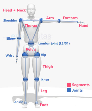
A human model describes the number of segments that compose the body, and the location of the center of gravity and the weight of each segment. This set of data is called the inertial parameters of the human model. The segmentation of the body can be carried out in multiple ways, although usually 14 segments are used (Head+Neck, Trunk, Thighs, Legs, Feet, Arms, Forearms and Hands). The segments are assumed to be non-deformable. Each segment is defined by two points in its longitudinal axis, which usually correspond to the ends of this axis: the proximal point (beginning of the segment) and distal point (end of the segment).
Other models divide the trunk into two, three or more segments: thorax, abdomen and pelvis (this is the model initially developed by Dempster (1955) and Plagenhoef (1962, 1971)). Other common modification is to simplify the model by reducing the number of segments, which implies assuming that some joints behave rigidly, losing mobility between adjacent limbs.
The model shown in the Figure 3 presents 15 segments, the trunk being divided into thorax and pelvis. The pelvis begins at the L5/S1 intervertebral space and end at the hips.
Figure 3:
Segments of a human model.
The study of the weight and the position of the center of gravity of each body segment has been approached using experimental techniques. These values depend on the amount of matter within the segments and their spatial distribution, which are unique to each individual.
Some authors have tried to obtain individualized inertial parameters for each person (Whitsett, 1963; Hanavan, 1964; Jensen, 1978; Hatze, 1980 and Yeadon 1990). However, the procedures to obtain them are costly and not very precise. Therefore, it is common to express the weight of each segment as a percentage of the total weight of the individual. There are several models of this type. The most commonly used is from the studies of Dempster (1955) and Clauser (1969), who obtained the data from the dismemberment of carcasses (Table 1).
Remember...
A human model describes the number of segments that compose the body, and the location of the center of gravity and the weight of each segment. This set of data is called the inertial parameters of the human model.
| SEGMENT | MASS | GC | Proximal point | Distal point |
|---|---|---|---|---|
| Head and neck | 7.3% | 46.40% | vertex | middle gonion |
| Trunk | 50.7% | 38.03% | suprasternal hollow | midpoint of the hips |
| Arm | 2.6% | 51.30% | acromion | radiale |
| Forearm | 1.6% | 38.96% | radiale | wrist |
| Hand | 0.7% | 82.00% | wrist | styloid 3rd finger |
| Thigh | 10.3% | 37.19% | hip | tibiale |
| Calf | 4.3% | 37.05% | tibiale | ankle |
| Foot | 1.5% | 44.90% | heel | finger 1º |
In Table 1 the MASS column indicates the mass of the segment as a percentage of the total mass of the subject. The CG column indicates the percentage, with respect to the total length of the corresponding segment, at which the center of gravity of the segment is located, measured from the proximal point.
Other studies, such as those of Drillis and Contini (1966) allow estimation of the length of the different body segments as a function of the individual's height (Table 2). It can be used when these values are unknown and direct measurement is impossible. The data on the length of the segments were obtained through measurements on living subjects, carrying out a statistical regression with respect to the height variable. In this way, the dimensions of each segment were obtained as a proportion of the individual's height. In general, correlations with r2>0.5 were found, except in the case of foot length and hand length where r2<0.5. It should be remembered that the values obtained are estimates, and that in any case direct measurement of lengths is preferable. Nevertheless, the use of correlations between height and body segment lengths results in a standard error of less than one centimeter. That is, 95% of the time, the actual and estimated lengths will differ by less than 2 centimeters.
Thus, it can be estimated that a person weighing 75 kilograms and measuring 175 cm. would have a forearm weighing 1.2 kilograms (75*0.016), with a length of 25.55 cm. (175*0.146), and whose center of gravity would be 9.95 cm. from the radial.
SEGMENT % STATURE Hand 10.8% Torax 28.8% Arm 18.6% Forearm 14.6% Pelvis 4.5% Thigh 20.0% Calf and foot 28.5% Table 2:
Estimation of the length of body segments.
Using a human model and its inertial parameters it is possible to calculate the moments generated by a handled load and the weight of the body segments in each joint, and evaluate the risk of causing musculoskeletal injuries. This assessment involves comparing the generated moments with the maximum recommended ones.
As mentioned earlier, the degree of muscle stretch varies with movement, and so does the capacity of the muscles to produce force. Additionally, the movement produces changes in the lever arm of the forces.
Some studies determine the maximum muscular forces depending on postures and types of movements. This makes it possible to know the maximum moments that the muscles of each joint can generate in each posture. Essentially, to avoid any injury when someone attempts to pull, push, or lift a load with maximum effort, the moments generated by the handled load and the weight of the body segments should be equal or lesser than the moments that the muscles involved in the movement can generate.
Therefore, there is a muscle force moment that should not be exceeded by the moments generated by external loads. A biomechanical model establishes the maximum effort possible in each joint depending on the posture and type of movement. One of the first models was developed by Chaffin (1969). It is a static and coplanar model (sagittal plane) designed to study movements involved in load handling. This model states that the following condition must be met:
- Sj < Mj/L < Sj
where:
-Sj is the maximum moment that the joint j can withstand when the extensor muscles are acting.
Sj is the maximum moment that the joint j can withstand when the flector muscles are acting.
Mj/Lis the moment acting on each joint j due to the external handled load L and the weight of the body segments supported by that joint j.
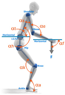
As previously mentioned, calculating Mj/L for each joint can be done by applying the equations of equilibrium. To calculate Sj and -Sj testing with different types of subjects is required. Estimating these values involves considering numerous factors, including posture, the operator's physical constitution, time, and the duration of the posture (the longer the posture is adopted, the lower the maximum recommended moment will be). A study of this type was conducted by Stobbe in 1982 taking these factors into account and following the appropriate methods. As already mentioned, the force moments of the muscles vary according to the joint's range of rotation. Therefore, the angles between segments must be known in order to calculate Sj and -Sj. In the model used in Ergoniza the angles must be measured as shown in Figure 4.
Studies by Clarke (1966), Schanne (1972) and Burggraaf (1972) determined the values of Sj and -Sj. The data were taken from a sample of school-age subjects of both sexes, so they cannot be considered representative of the industrial population. For that reason, Chaffin (1999) uses data obtained by Stobbe (1982), drawn from male and female workers in industry, to adjust the expected mean values and estimate a coefficient of variation around the mean.
Remember...
A Biomechanical Analysis consists of comparing the moments generated in the joints in a given posture with a given handled load with the maximum moments thah muscles can generate under those conditions.
Figure 4:
Measurement of angles between segments.
Table 3 shows some of the equations proposed by Chaffin for the calculation of Sj and -Sj.
| Effort | Primary and Adjacent Joint | Sj* (Nm) | G (Gender Adjustment) | Coefficient of Variation | ||
|---|---|---|---|---|---|---|
| Male | Female | Male | Female | |||
| Elbow flexion | Elbow/shoulder | Se = [336.29 + 1.544αe - 0.0085 αe2 - 0.5αs][G] | 0.1913 | 0.1005 | 0.2458 | 0.2629 |
| Elbow extension | Elbow/shoulder | -Se = [264.153 - 0.575αe - 0.425αs][G] | 0.2126 | 0.1153 | 0.2013 | 0.3227 |
| Shoulder flexion | Shoulder/Elbow | Sh = [227.338 + 0.525αe - 0.296αs][G] | 0.2845 | 0.1495 | 0.2311 | 0.2634 |
| Shoulder extension | Shoulder | -Sh = [204.562 - 0.099αs][G] | 0.4957 | 0.2485 | 0.3132 | 0.3820 |
| . | ... | ... | ... | ... | ... | ... |
| . | ... | ... | ... | ... | ... | ... |
Let's assume we want to determine the maximum moment the elbow can withstand in the position depicted in Figure 1. First, it is essential to identify whether the active muscles are the forearm's flexors or extensors. Maintaining the forearm in the posture shown in this figure necessitates the action of the biceps, brachialis, and brachioradialis muscles, which are the forearm's flexor muscles. Consequently, this is an elbow flexion.
As seen in the first row of Table 3, the primary and adjacent joints for elbow flexion are the elbow and shoulder. Thus, we must determine the angles αe and αs (in sexagesimal degrees), as illustrated in Figure 4. The values of these angles should be input into the corresponding equation:
Se=[336.29 + 1.544αe-0.0085 αe2 -0.5αs][G]
together with that corresponding to G, which for a man takes the value of 0.1913 according to Table 3. Considering that αe = 90º and αs = 0º we obtain that Se= 77.74 Nm.
Hence, the maximum moment not to be exceeded at the elbow in the analyzed posture for an individual with the given height and weight is 78.19 Nm. However, not all individuals of the same build will share the same limit. The calculated value represents the mean Se, which is the maximum limit for 50% of individuals with these characteristics. Assuming that this limit follows a normal distribution, the calculated Se serves as the mean of this distribution. To estimate the standard deviation (SD), the Coefficient of Variation (found in the last column of Table 3) is multiplied by the mean value (keeping in mind that ± 1 SD covers 68% of the population and ± 2 SD covers 95%, assuming a normal distribution of the data).
By knowing the mean and standard deviation of the maximum moment distribution, it is possible to determine the percentage of the population protected when a given load is sustained, or the maximum load to be sustained for a specific percentage of the population to be protected.
On the other hand, the calculated value is the maximum recommended for punctual postures and efforts of short duration. This value should be reduced if the efforts are performed for long or frequent periods. The recommended limits will depend on the duration of the action and its repetitiveness. Depending on them, the efforts will be classified as follows:
Static effort (maintained for more than one minute).
Efforts that are cyclically repeated (more than once every 5 minutes)
Efforts repeated less than once every 5 minutes
The Table 4 shows the percentage of the maximum load that should not be exceeded depending on the repetitiveness and duration
Remember...
The calculated value is the maximum recommended for punctual postures and efforts of short duration. This value should be reduced if the efforts are performed frequently or for long periods. The recommended limits depend on the duration of the action and its repetitiveness.
Repetitiveness Duration <= 1 hour > 1 hour Static effort 5% 2% Efforts that are cyclically repeated more than once every 5 minutes 14% 10% Efforts with a frequency of less than once every 5 minutes 70% 50% Table 4
Percentage of maximum recommended load as a function of repetitiveness and duration of the effort.
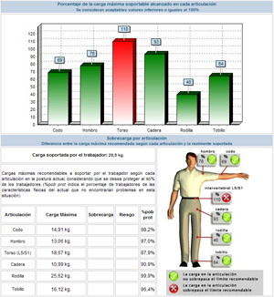
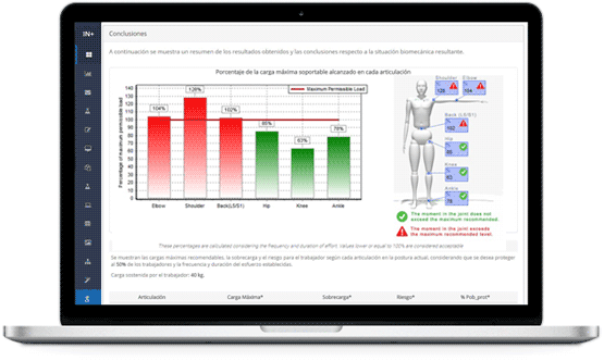
The application of the described model for assessing stresses in various joints can be a complex procedure without the aid of a computer tool. The calculation tool provided by Ergoniza facilitates the application of the model and the calculations, offering results such as: stress level in each joint, maximum recommended load, percentage of protected population, as well as posture stability, potential for slipping, and the possibility of the worker overturning under the supported loads.
To proceed with the calculations, the following data on the task must be collected:
Worker's gender.
Worker's height.
Worker's weight.
Angles of the body segments in the analyzed posture.
Weight of the load held or force exerted.
Whether the load is held with one or two hands.
Duration of the efforts.
Frequency of the efforts.
In addition, if it is desired to calculate the possibility of worker slippage due to the adopted posture and sustained load, the coefficient of friction between the footwear and the floor must be known.
Using this data, the software will calculate the stress and moments generated in each joint and compare them with the maximum permissible in that posture obtained from the above model, modified according to the duration and frequency of the effort, and the percentage of the population to be protected. The program will determine the existing risk based on the difference between the acting moment and the permissible moment in each joint.
Figure 5:
Results of the method.
Before applying the method, it is crucial to understand the simplifications assumed in its development and the limitations of its application. As mentioned in the previous sections, human models estimate the length of the body segments, the weight, the position of the center of gravity, the maximum recommended moment in each the joints as well as their distribution around the mean, among others. Although all these models have been endorsed and validated in the scientific literature on the subject, and are widely used and accepted within the scientific community, they remain estimates of reality. The fact that, for example, 95% of the time the actual and estimated length of a body segment differ by less than 2 centimeters does not imply that there is a certain margin of error.
Regarding physical calculations, the following assumptions have been made::
All body segments are considered rigid, with no changes in mass, density, or shape depending on posture.
The centers of mass of the segments do not change position relative to the proximal or distal ends of the segment.
The radius of gyration of each segment remains constant during movement.
The load's point of application is located at the center of the palm of the hand.
The load does not generate moments in the body.
No part of the body is supported, with the operator standing only on their feet.
If the load is supported by only one hand, the non-lifting arm is considered to be in the same position as the arm exerting the force.
Lastly, it is essential to remember that the assumed model assesses isometric, static, and coplanar (sagittal plane) efforts in two dimensions. As a static model, it serves as a particularly useful tool for designing and evaluating stresses in two dimensions, where the acceleration effect of the load and body segments is negligible. For analyzing slow load handling movements, the model can be applied by describing the activity as a series of static postures, analyzing them separately, and assuming that the inertial effects caused by acceleration are negligible in any case.
Failing to consider these simplifications and limitations may result in inaccurate outcomes.
Chaffin, d.b., Anderson, g.b.j. & Bernard, j.m., 2006, Occupational Biomechanics (4ª Edición). John Wiley & Sons. Hoboken, New Jersey.
Chandler,R.F.; Clauser,C.E.; McConville,J.T.; Reynolds,H.M. & Young,J.W.,1975. Investigation of inertial porperties of the human body. AMRL-TR-74-137, AD-A016-485, DOT-HS-801-430. Aerospace Medical Research Laboratories, Wright-Patterson Air Force Base, Ohio.
Clauser,C.E.; McConville,J.T. & Young,J.W., 1969. Weight, volume and center of mass of segments of the human body. AMRL-TR-69-70. Aerospace Medical Research Laboratory, Wright-Patterson Air Force Base, Ohio.
Dempster,W.T., 1955. Space requirements of the seated operator. WADC-55-159, AD-087-892. Wright-Patterson Air Force Base, Ohio.
Diego-Mas, J.A., Poveda-Bautista, R. & Garzon-Leal, D.C., 2015. Influences on the use of observational methods by practitioners when identifying risk factors in physical work. Ergonomics, 58(10), pp. 1660-70.
Drillis,R.J. & Contini,R.,1966. Body segment parameters. BP174-945, Tech.Rep. Nº 1166.03, School of engineering and science, New York University, New York
Garg, A, Chaffin, D.C. and Herrin, G.D.,1978, Prediction of metabolic rates for manual material handling jobs, American Industrial Hygiene Association Journal, 39, pp. 661-764.
Niosh,1981, Work practices guide for manual lifting. NIOSH Technical Report nº 81-122, National Institute for Occupational Safety and Health
Roebuck, J.A., Kroemer K.H.E. & Thomsnon W. G., 1975, Engineering anthropometry methods. Wiley-Interscience, New York.
Waters, T.R., Putz-Anderson, V. & Garg, A, 1994, Applications manual for the revised Niosh lifting equation. National Institute for Occupational Safety and Health. Cincinnaty. Ohio
Diego-Mas, Jose Antonio. Coplanar static biomechanical analysis Ergonautas, Universidad Politécnica de Valencia, 2023. Available online: https://www.ergonautas.upv.es/ergoniza/app_en/land/index.html?method=biomecanica
A cloud based software that integrates more than 20 tools for managing the ergonomics of the workstations in your company.
Evaluate all ergonomic risk factors of the workstations in your company: inadequate postures, repetitive movements, load handling, thermal environment...
Generate fully customizable reports in Microsoft Word or Adobe Pdf format.

Use Artificial Intelligence for automated posture detection from photographs or videos, or to automatically interpret your assessment results and obtain recommendations.
In a multiuser environment so that your company can have access to your data everywhere.
You only need a free account on Ergoniza
ERGONIZA allows you to use Artificial Intelligence for postural load assessment. Automatically capture workers’ postures from a photograph or a video and obtain an automated evaluation of the risk associated with inadequate or forced postures.
The Artificial Intelligence of ERGONIZA interprets the results of your assessments and automatically generates conclusions and recommendations.
AI in actionERGONIZA helps you manage the ergonomics of the workstations of your companies. Evaluate all the risk factors present in the workstations, manage the evaluations, and obtain editable and customizable reports.
You only need to register as a user of ERGONIZA to start testing.
Sign UpUnlock the full potential of Ergoniza. By becoming a Pro User you'll have access to all of Ergoniza and be able to use all of the online software without restrictions or time limits. You'll be able to use the results of evaluation methods and tools in your professional activity. You'll be able to print the results reports in pdf or Word and save your studies in files to open them later.
To register as a Pro user, you must first login to Ergoniza.
(*) In European Union countries, the price will be increased with the corresponding VAT.
(**) The price in american dollars has been calculated at the current exchange rate and may vary.
is a web by . Ergonautas is the specialized website in occupational ergonomics and ergonomic assessment of workstations at the . Ergonautas aims to be a useful support tool for the Occupational Risk Prevention and Ergonomics professional and people in training, providing rigorous technical information on occupational ergonomics, online tools for its application, research, training, and participation forums.
Ergonautas is formed by a large human team. In addition to technicians and programmers, the Ergonautas team is made up of researchers and professors from the Polytechnic University of Valencia. The team, led by José Antonio Diego Más, is at the forefront of research and teaching in ergonomics, teaching in official degrees and master's degrees, and developing research projects in the field of ergonomics and new technologies oriented towards humans.
If you need to know more, get in touch with Ergonautas
Or follow us on Linkedin
- - -
© 2006 - Universidad Politécnica de Valencia